Training T-SNE Clustering
T-SNE is mostly useful for data visualization.
T-SNE plots can be misleading, typically cluster size have no true meaning and distances cannot be trusted, read https://distill.pub/2016/misread-tsne/ for more detailed information.
Data format
T-SNE use CSV data format, see the relevant CSV data section above.
Training for a T-SNE visualization
Using DD platform, from a JupyterLab notebook, start from the code on the right.
T-SNE notebook snippet:
tsne_mnist = TSNE_CSV(
    'tsne_mnist',
    training_repo = 'https://deepdetect.com/dd/datasets/mnist_csv/mnist_test.csv',
    host='deepdetect_training',
    port=8080,
    model_repo='/opt/platform/models/training/examples/test_tsne/',
    iterations = 5000,
    perplexity = 30
)
tsne_mnist
Building a T-SNE plot after training has completed:
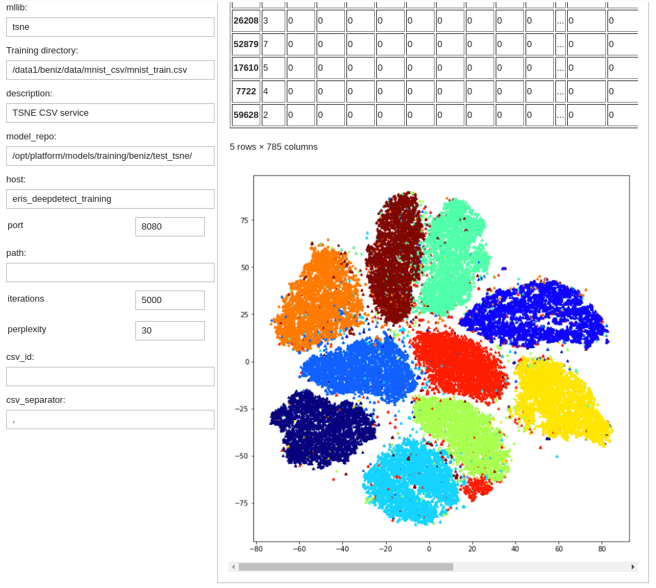
tsne_mnist.plot()
Screening the T-SNE plot with per-class colours:
import pandas as pd
df_orig = pd.read_csv("/path/to/mnist_train.csv")
tsne_mnist.plot(s=10, marker='^', c=df_orig.label, cmap='jet')
This runs a T-SNE compression job with the following parameters:
T-SNE creates a 2D point representation from a set of points, and does not save a reusable model on disk. In other words it is only usable on the training set points and cannot generalize to more points.
tsne_mnistis the example job name
Job names must be unique, replace `tsne_mnist` with your own
Using job names that reflect your experiments is good practice, e.g. `city_pspnet_iter75k_dice_weighted_amsgrad`
training_repospecifies the location of the dataiterationsspecifies the maximum number of iterationsperplexityis related to the number of nearest neighbors used to learn the underlying manifold.
Once training has completed, the following steps on the right can be used to generate the plot below: